Active Learning with Nvidia TLT
How to go from a quick prototype to a production-ready object detection system using active learning and Nvidia TLT
One of the biggest challenges in every machine learning project is to curate and annotate the collected data before training the machine learning model. Oftentimes, neural networks require so much data that simply annotating all samples becomes an insurmountable obstacle for small to medium sized companies. This tutorial shows how to make a prototype based on only a fraction of the available data and then iteratively improve it through active learning until the model is production ready.
Active learning describes a process where only a small part of the available data is annotated. Then, a machine learning model is trained on this subset and the predictions from the model are used to select the next batch of data to be annotated. Since training a neural network can take a lot of time, it makes sense to use a pre-trained model instead and finetune it on the available data points. This is where the Nvidia Transfer Learning Toolkit comes into play. The toolkit offers a wide array of pre-trained computer vision models and functionalities for training and evaluating deep neural networks.
The next sections will be about using Nvidia TLT to prototype a fruit detection model on the MinneApple dataset and iteratively improving the model with the active learning feature from LightlyOne, a computer vision data curation platform.

Why fruit detection?
Accurately detecting and counting fruits is a critical step towards automating harvesting processes. Fruit counting can be used to project expected yield and hence to detect low yield years early on. Furthermore, images in fruit detection datasets often contain plenty of targets and therefore take longer to annotate which in turn drives up the cost per image. This makes the benefits of active learning even more apparent.
Why MinneApple?
MinneApple consists of 670 high-resolution images of apples in orchards and each apple is marked with a bounding box. The small number of images makes it a very good fit for a quick-to-play-through tutorial.
Let’s get started
This tutorial follows its Github counter-part. If you want to play through the tutorial yourself, feel free to clone the repository and try it out.
Upload your Dataset
To do active learning with LightlyOne, you first need to upload your dataset to the platform. The command lightly-magic trains a self-supervised model to get good image representations and then uploads the images along with the image representations to the platform. Thanks to self-supervision, no labels are needed for this step so you can get started with your raw data right away. If you want to skip training, you can set trainer.max_epochs=0. In the following command, replace MY_TOKEN with your token from the platform.
For privacy reasons, it’s also possible to upload thumbnails or even just metadata instead of the full images. See this link for more information.
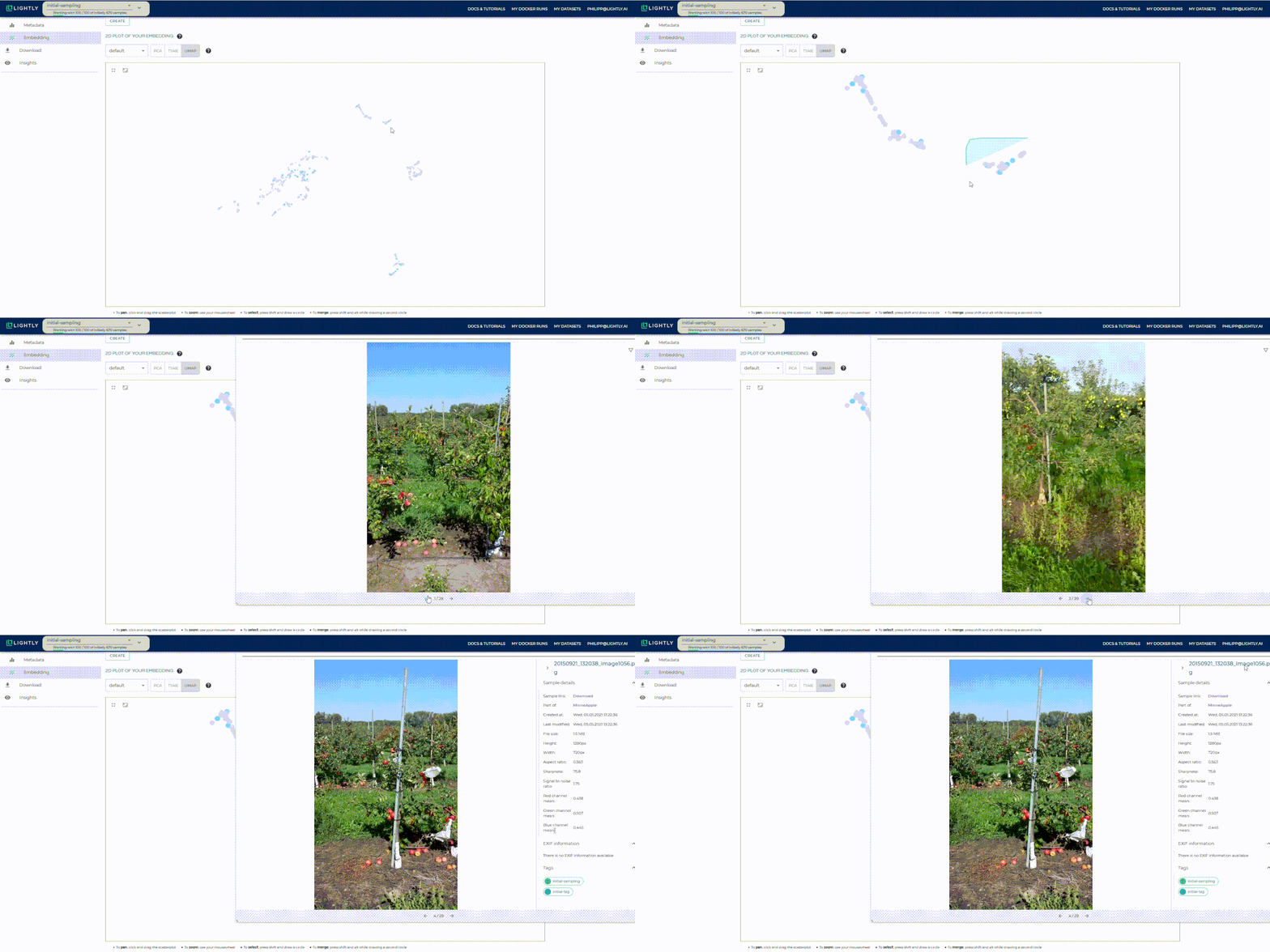
Once the upload has finished, you can visually explore your dataset in the LightlyOne Platform. You will likely detect different clusters of images. Play around with it and see what kind of insights you can get.

Initial Sampling
Now, let’s select an initial batch of images for annotation and training.
LightlyOne offers different sampling strategies, the most prominent ones being CORESET and RANDOM sampling. RANDOM sampling will preserve the underlying distribution of your dataset well while CORESET maximizes the heterogeneity of your dataset. While exploring our dataset in the LightlyOne Platform, we noticed many different clusters. Therefore, we choose CORESET sampling to make sure that every cluster is represented in the training data.
To do an initial sampling, you can use the script provided in the Github repository or you can write your own Python script. The script should include the following steps.
Create an API client to communicate with the LightlyOne API.
Create an active learning agent which serves as an interface to do active learning.
Finally, create a sampling configuration, make an active learning query, and use a helper function to move the annotated images into the data/train directory.
The query will automatically create a new tag with the name initial-selection in the LightlyOne Platform.
Training and Inference
Now that we have our annotated training data, let’s train an object detection model on it and see how well it works! Use the Nvidia Transfer Learning Toolkit to train a YOLOv4 object detector from the command line. The cool thing about transfer learning is that you don’t have to train a model from scratch and therefore require fewer annotated images to get good results.
Start by downloading a pre-trained object detection model from the Nvidia registry.
Finetuning the object detector on the sampled training data is as simple as the following command. Make sure to replace YOUR_KEY with the API token you get from your Nvidia account.
Now that you have finetuned the object detector on your dataset, you can do inference to see how well it works.
Doing inference on the whole dataset has the advantage that you can easily figure out for which images the model performs poorly or has a lot of uncertainties.
Below you can see two example images after training. It’s evident that the model does not perform well on the unlabeled image. Therefore, it makes sense to add more samples to the training dataset.

Active Learning Step
You can use the inferences from the previous step to determine which images cause the model problems. With LightlyOne, you can easily select these images while at the same time making sure that your training dataset is not flooded with duplicates.
This section is about how to select the images which complete your training dataset. You can use the active_learning_query.py script again but this time you have to indicate that there already exists a set of preselected images and point the script to where the inferences are stored.
Note that the n_samples argument indicates the total number of samples after the active learning query. The initial selection holds 100 samples and we want to add another 100 to the labeled set. Therefore, we set n_samples=200.
Use CORAL instead of CORESET as a sampling method. CORAL simultaneously maximizes the diversity and the sum of the active learning scores in the sampled data.
The script works very similarly to before but with one significant difference: This time, all the inferred labels are loaded and used to calculate an active learning score for each sample.
The rest of the script is almost the same as for the initial selection:
Re-training
You can re-train our object detector on the new dataset to get an even better model. For this, you can use the same command as before. If you want to continue training from the last checkpoint, make sure to replace the pretrain_model_path in the specs file by a resume_model_path.
If you’re still unhappy with the performance after re-training, you can repeat the training, prediction, and active learning steps again — this is then called the active learning loop. Since all three steps are implemented as scripts, iterations take little effort and are a great way to continuously improve the model.
— — — — — — — — — — — — — — — — — — — — — — — — — — — — — —
Philipp Wirth
Machine Learning Engineer
lightly.ai

.png)


.png)


-min.png)

