Embeddings in Machine Learning: An Overview
Table of contents
Embeddings are vector representations that encode the meaning and relationships of data like words or images. They map items into continuous spaces where similar entities are close, powering NLP, vision, and recommendation systems.
Here is an overview of embedding spaces and their role in multi-modal learning:

- What are embeddings in machine learning?
Embeddings are numerical vector representations of data (words, images, etc.) that capture semantic meaning and relationships. Instead of using sparse identifiers (like IDs or one-hot encodings), embeddings map items into a continuous vector space where similar items are positioned closer together and dissimilar ones far apart.
- How do embeddings work in ML?
Embeddings are learned by neural networks or algorithms that compress high-dimensional or categorical data into lower-dimensional vectors. During training, the model adjusts the embedding values so that meaningful patterns emerge – for example, words that appear in similar contexts end up with similar vectors. This process often uses an embedding layer in a neural network, which transforms input tokens (e.g. word IDs) into dense vectors that the model can process.
- Why are embeddings useful in machine learning?
They enable ML models to interpret complex data more effectively by encoding semantic relationships and reducing dimensionality. For instance, word embeddings place synonyms near each other in vector space, helping NLP models understand context and meaning. Embeddings also make computations more efficient (dense low-dimensional vectors instead of huge sparse vectors) and allow similarity searches – e.g., finding similar images or documents by comparing embedding vectors.
- What is an embedding layer in a neural network?
An embedding layer is a component of neural networks (especially in NLP and recommendation systems) that maps discrete inputs to continuous vectors. It’s essentially a lookup table of vectors that gets learned during training. For example, in a language model, an embedding layer takes each word’s ID and outputs a trained vector for that word, which then feeds into the network’s hidden layers. This allows the model to learn which words (or categories) are similar based on training data, rather than relying on arbitrary indices or one-hot encodings.
- How are embeddings used in NLP and computer vision?
In natural language processing, word embeddings (like Word2Vec or BERT embeddings) encode the meanings of words or sentences, powering tasks like translation, sentiment analysis, and search by semantic similarity. In computer vision, image embeddings (features extracted by CNNs or vision transformers) represent images in vector form, enabling tasks such as image retrieval, object detection, and face recognition by comparing image vectors. In both cases, embeddings allow the model to compare inputs in terms of meaning or content rather than raw pixels or text.
Introduction
Machine learning (ML) algorithms are based on mathematical operations and work only with numerical data. They cannot understand raw text, images, or sound data directly.
Embeddings are a key technique to feed complex data types into models. It turns words, images, or audio data into numbers so that machines can understand.
In this guide, we’ll cover:
- What Are Embeddings in Machine Learning?
- Why Embeddings Matter (Benefits and Importance)
- How Embeddings Are Created and Trained.
- Applications of Embeddings in Machine Learning
- How Can Lightly AI Help With Embedding Requirements
Embeddings are only as good as the data that shapes them. At Lightly, we help ML engineers to create high-quality embeddings without wasting time or resources through:
- LightlyOne: Curate the most representative and diverse samples in your dataset. It ensures that data for creating embeddings covers all the important variations while avoiding redundant data.
- LightlyTrain: Pretrain custom embedding models with self-supervised learning. By first training on your domain-specific unlabeled data you can obtain embeddings that generalize better to your downstream tasks.
Try them for free and start building better embeddings today!
See Lightly in Action
Curate and label data, fine-tune foundation models — all in one platform.
Book a Demo
What Are Embeddings in Machine Learning?
Embeddings are dense vector representations of real-world objects and relationships in a continuous vector space.
They place high-dimensional data into a low-dimensional space while preserving semantic relationships (similar items are placed closer together).
Simply put, an embedding distills the richness of complex information into compact, meaningful forms. And it lets models share learnings across similar items rather than treating them as unique categories.
For example, in the image below, the vectors for cat and kitten, or adult and child, are close together in the embedding space because of their semantic similarity. And, if there is a vector for a car, it would be far apart due to dissimilarity.
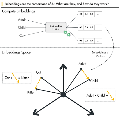
- In natural language processing (NLP), words or sentences are embedded so that terms with similar meaning lie close together in embedding space.
- In computer vision, image embeddings represent images as vectors so that visually or semantically similar images cluster in vector space.
- For graph embeddings, nodes in a knowledge graph become vectors where nodes with similar neighborhoods or connectivity are near each other.

Why Embeddings Matter: Benefits and Importance
Since embeddings enable computers to understand the complex relationships between words and other objects, just as humans do, they are foundational for artificial intelligence (AI).
Let's discuss the benefits they offer in practice.
Capturing Semantic Relationships
Embeddings capture the syntactic (grammatical) and semantic relationships between objects.
At the core, they map data points so that the geometric distances between numerical vectors reflect their real-world relationships.
For example, words with similar meanings or images with comparable visual features are positioned closer together.

Dimensionality Reduction
Real-world data can have tens, hundreds, or thousands of features or attributes. Processing such high-dimensional and often sparse data demands more computing power.
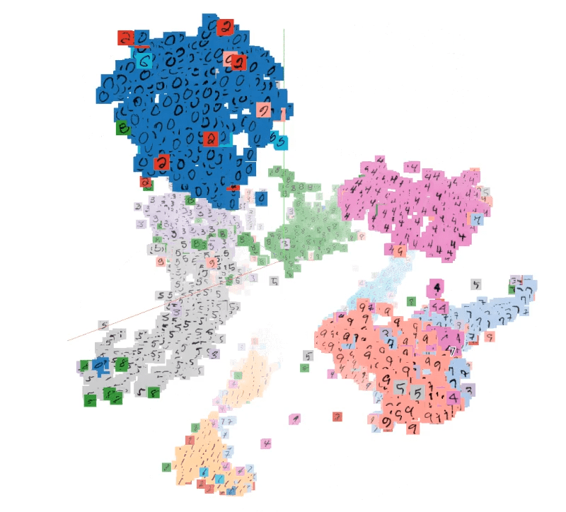
Embeddings solve this by compressing the data into a denser dimensional space, preserving important information while filtering out noise.
Enabling Similarity Search
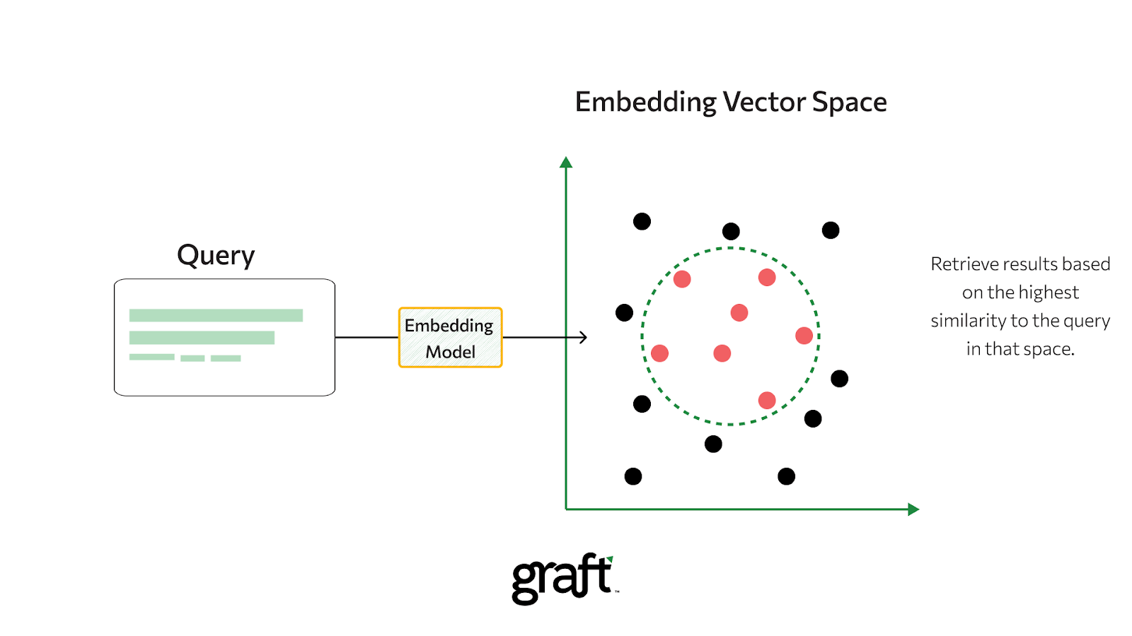
Since similar items are placed close together, embeddings are great for tasks that involve finding similarities.
We can easily see how close two items are using distance metrics like Euclidean distance or cosine similarity. And this calculation is the foundation for many applications, including semantic search, product recommendations, and finding duplicate data.
Improved Generalization
Models built on top of embeddings often generalize better to new examples. As embeddings are learned from data, they capture underlying patterns that hand-crafted features might miss.
For instance, if two words had never appeared in the same context in training, a good embedding model might still place them near each other if they share similar contexts elsewhere.
How Are Embeddings Created?
Various deep learning models can generate embeddings that understand the context and semantics of your input. But the choice varies depending on the type of data input.
Thus, it is fundamental to understand your data and what you need from it before picking an embedding model.
To create numerical representations of data, we usually have two main options: training our own models (whether using an embedding layer or a self-supervised learning method) or using pretrained models.
Using an Embedding Layer
The deep neural networks start with an embedding layer (a type of hidden layer that acts as a lookup table) that maps discrete inputs (like word indices or item IDs) into dense vectors in a continuous vector space.
The embedding layer is simply a trainable weight matrix of size (vocab_size × embedding_dim). Vocab_size is the number of unique discrete items, and embedding_dim is the embedding dimension you choose.
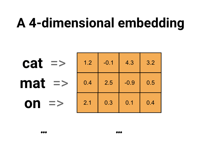
When the network gets an input (like word indices or item IDs), it selects the corresponding row of this matrix as the embedding (dense vector that now represents that item).
Initially, these vectors are random. But as the network trains, the values in this matrix are updated to minimize the model's error.
Over time, the layer learns to assign similar vectors to items that behave similarly, creating a meaningful and efficient representation of the data.
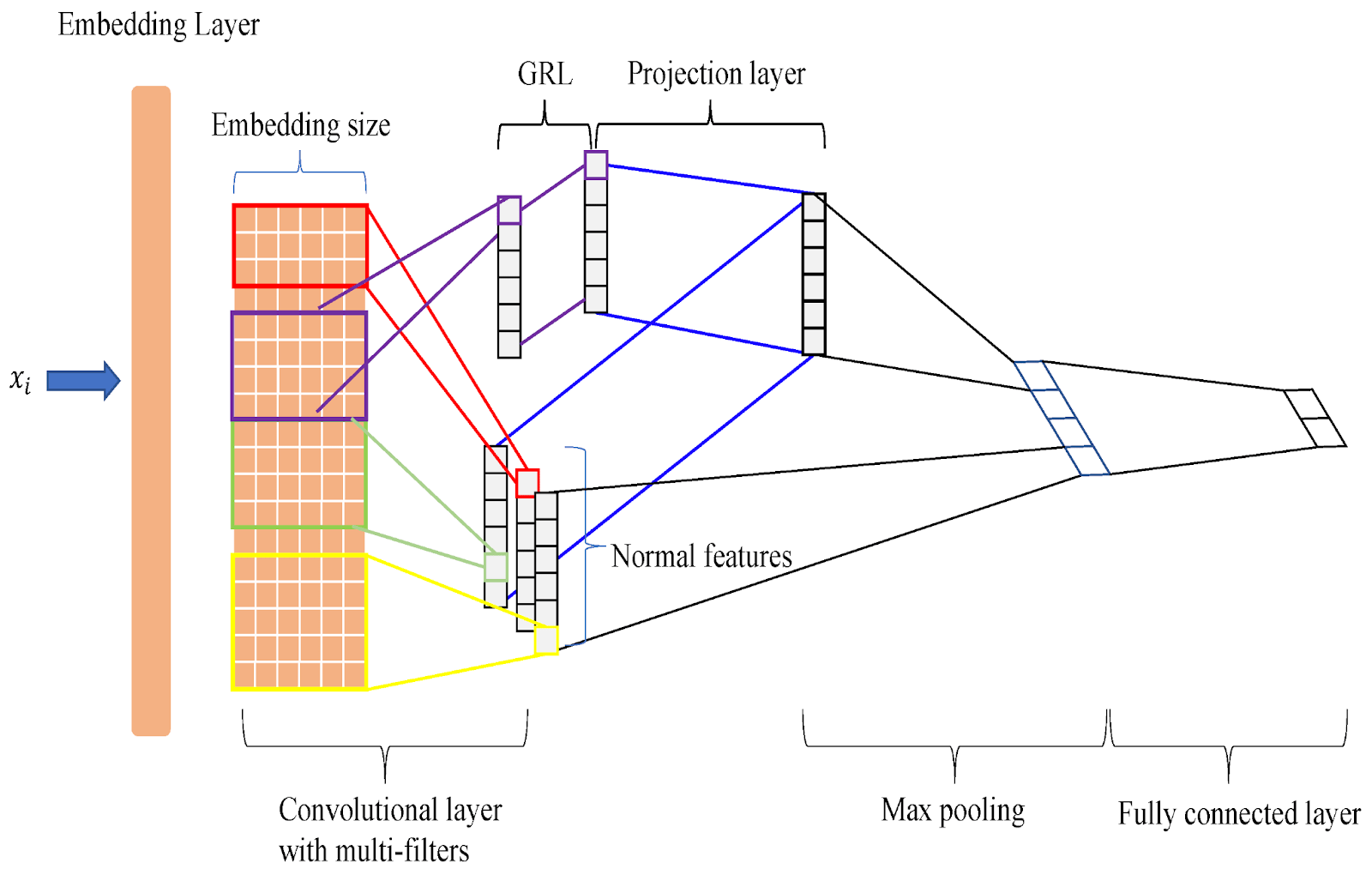
However, training an SOTA embedding model from scratch requires a lot of labeled datasets and enormous computational power. Instead, you use pretrained models (also known as foundation models) for transfer learning.
Using Pre-trained Models
Pretrained models (general-purpose models) have already been trained on web-scale data. You can use them "off-the-shelf" to generate high-quality embeddings instantly.
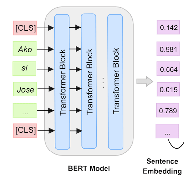
- For Text, transformer models like BERT or RoBERTa provide strong contextual embeddings that understand the nuances of language (contextual relationships).
- For Images, you can use pre-trained CNNs like ResNet or EfficientNet for extracting rich visual feature vectors.
- For multimodal data, the CLIP model provides a shared embedding space for both text and images, enabling cross-modal search.
Using Self-Supervised Learning
Sometimes, general-purpose embeddings are not enough, especially when we have specialized data like medical scans or financial documents.
In these cases, you can train your own embeddings. The most effective way to do this without expensive labeled data is through self-supervised learning (learning without labels).
It enables models to learn embeddings by utilizing the structure of the data itself as supervision, rather than relying on explicit labels.
Self-supervised learning methods and models include:
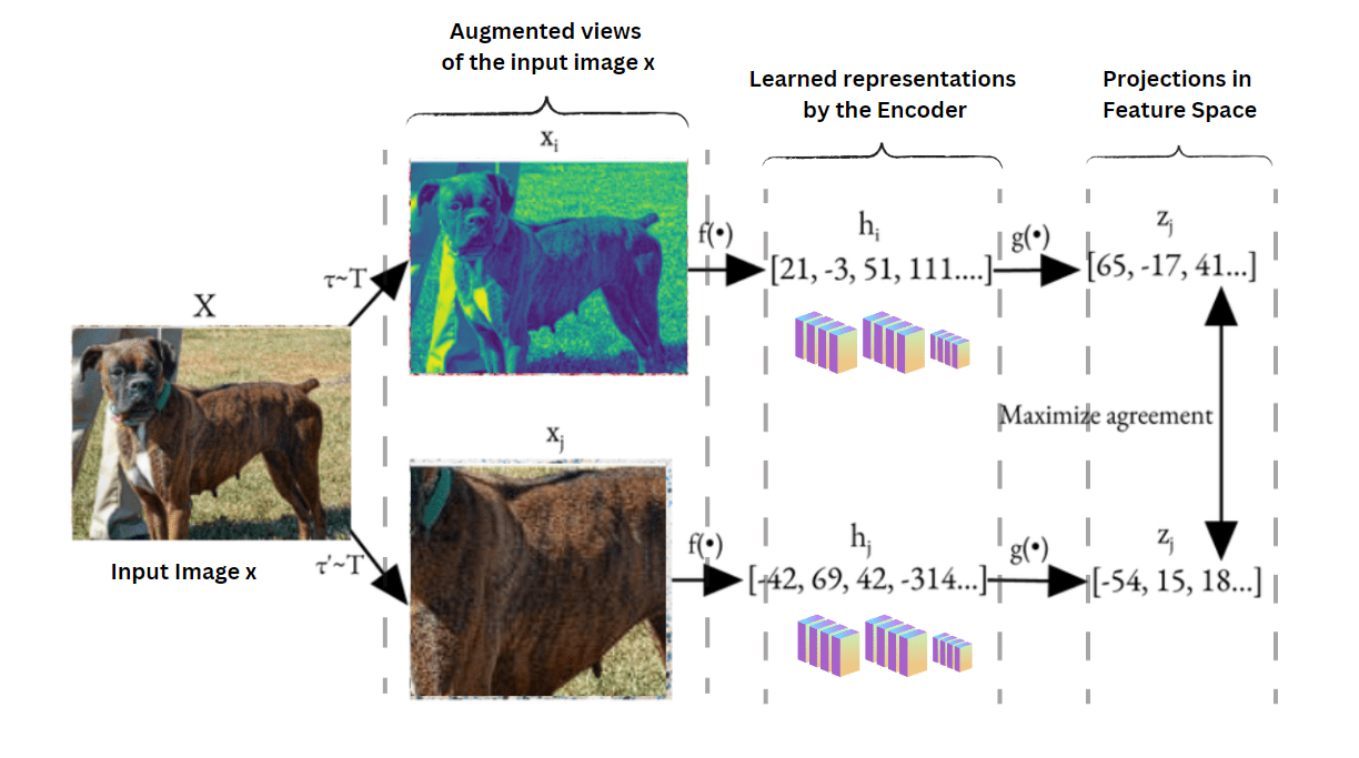
- Contrastive Learning, for example, in images, models like SimCLR or MoCo train embeddings so that random augmentations of the same image are pulled together in vector space, while other images are pushed apart.
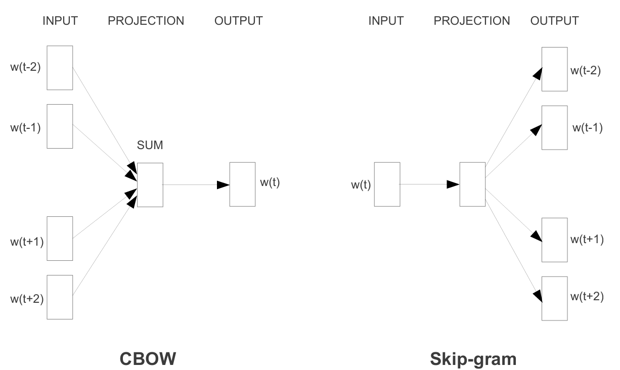
- Word2Vec (Skip-gram, CBOW) model predicts nearby context words. During training, it adjusts word vectors so that words appearing in similar contexts end up with similar embeddings.
- GloVe (Global Vectors) is a count-based method. It builds a global co-occurrence matrix of words from a large text corpus and then factorizes it to create word embeddings that capture the global statistical structure in vector space.

Implementing self-supervised pipelines yourself for computer vision can be complex. Using LightlyTrain, it's as simple as writing a couple lines of code, and you end up with custom high-quality vision embeddings from your unlabeled data.
See how effortlessly we can train a ResNet18 model (we also support models from different libraries) using the SimCLR method. Other pretraining techniques LightlyTrain supports include DINO and DINOv2.
import lightly_train

if __name__ == "__main__":
	lightly_train.train(
		out="out/my_experiment",
		data="my_data_dir",
		model="torchvision/resnet18",
		method="simclr",
)
Embeddings in NLP: Word, Sentence, and Document Embeddings
In natural language processing, embeddings represent words, phrases, or entire texts as vectors. Two broad categories of embeddings are static and contextual embeddings.
Static embeddings keep each token (word or subword) fixed with one vector regardless of context. For example, the word bank has the same vector whether used in river bank or bank account. They are fast and simple, but cannot handle words with multiple meanings.
While contextual embeddings give different representations (embeddings) to the same word in different sentences.
💡Pro Tip: If you work with embeddings for multilingual tasks, our Swiss-German LLMs article provides a concrete example of building meaningful representations for a dialect with limited training data.
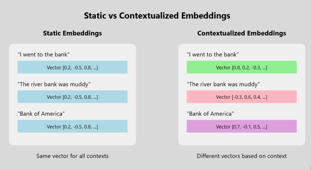
Here's a table summarizing the differences between the two:
Embeddings in Computer Vision: Image Embeddings
Just as we can convert words into vectors, we can do the same for images. An image embedding is a dense vector that captures the visual content of an image, such as its colors, shapes, textures, and the objects it contains.

Pre-trained CNNs, like ResNet-50, are used to extract a high-dimensional vector (embedding) from an image's final layers.
The vector summarizes the image's content hierarchically, from basic edges and colors to high-level content (object identity, scene context)
We can also use Vision Transformers (ViTs) to create image embeddings. Instead of working with pixels through convolutions, ViTs look at an image as a series of smaller patches.
They then use the transformer architecture's attention mechanism to learn relationships between them, resulting in highly effective embeddings.
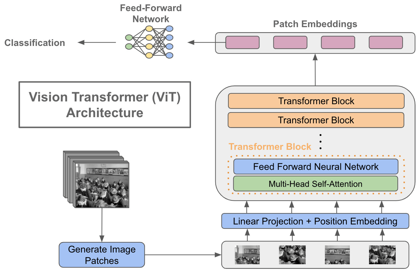
More recent approaches utilize self-supervised learning methods, such as contrastive learning for embedding creation.
The network learns to create similar embeddings for different augmented versions of the same image, while pushing apart embeddings from different images.
Once we have image embeddings, we can unlock a wide range of applications.
- Similarity and Retrieval: Image embeddings enable visual search by comparing the distance between vectors to find similar items. It can be used in applications such as face recognition (FaceNet) and image searching with text queries (CLIP).

- Data Curation and Clustering: Image embeddings allow you to explore your dataset’s embeddings to visualize clusters, spot outliers, and curate the most semantically diverse samples. Platforms like LightlyOne automate this curation process to enhance data quality.
💡Pro Tip: Zero shot performance depends heavily on rich embedding spaces. Our Zero-Shot Learning guide shows how strong representations enable models to handle unseen classes effectively.

- Object Detection and Recognition: Embeddings let modern object detection models like YOLO and Faster R-CNN use embedding-like feature vectors to identify and locate objects within an image.
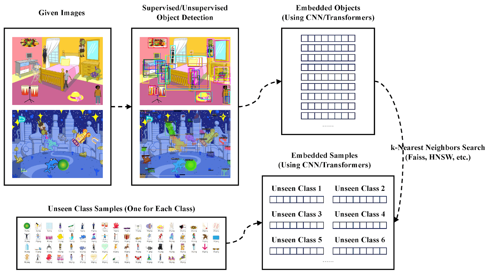
💡Pro Tip: Object detection backbones often rely on strong feature embeddings to localize and classify objects see our Object Detection guide for how detection models use learned embeddings to drive both localization and classification.
Graph and Other Types of Embeddings
Graph data (nodes and edges) can also be embedded in vector spaces. A graph embedding maps each node (or subgraph) to a vector so that the graph structure is preserved.
For example, in a social network, friends or friends-of-friends should have similar embeddings.
Methods like DeepWalk and node2vec create embeddings by performing random walks on the graph and then training Word2Vec on those walks.

Other domains' embeddings:
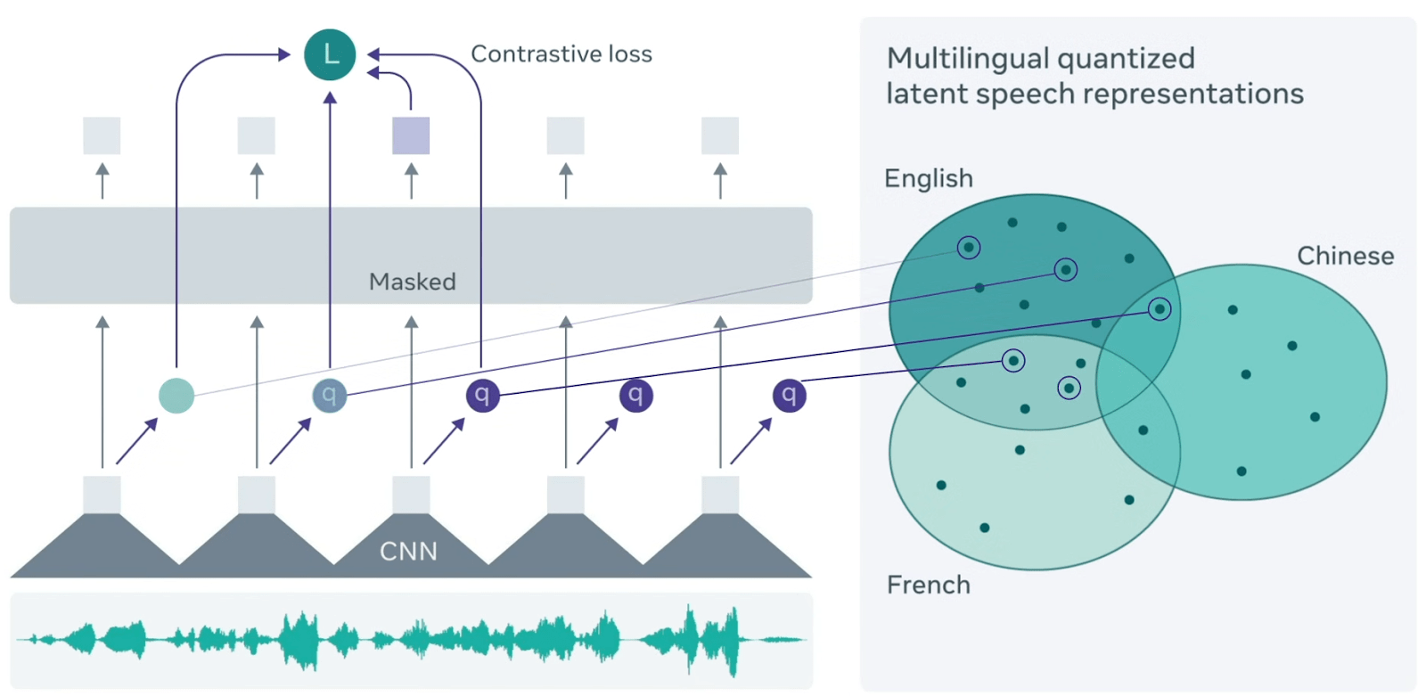
- Audio Embeddings: Audio (like speech or music) can be represented as embeddings to feed into machine learning models for tasks like speaker identification or music recommendation. Techniques include using models such as Wav2Vec (which learns speech representations) or utilizing embeddings from an audio classification network.
- Categorical Feature Embeddings: Even in structured or categorical data, fields (like user ID, product ID, zip code) are often handled with embeddings. Rather than one-hot encoding thousands of categories, an embedding layer turns each category into a small vector. This enables the model to learn category similarities.

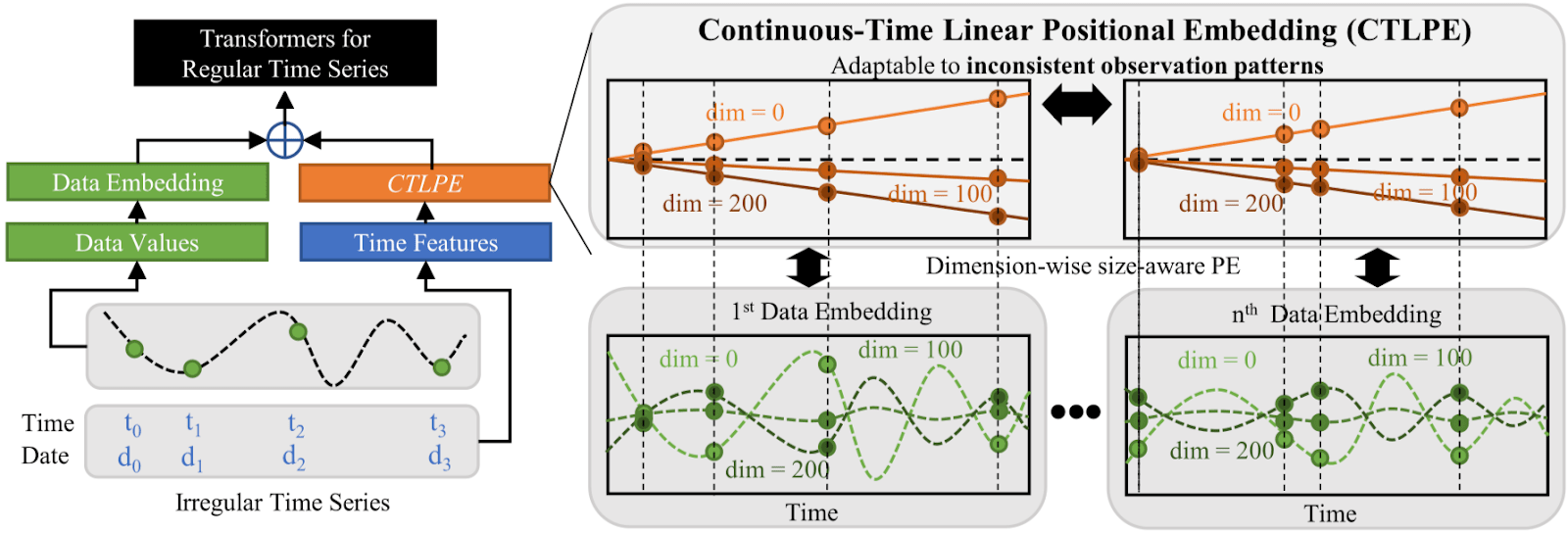
- Continuous Data Embeddings: Sequences can also be embedded using models like LSTMs or Transformers. For instance, an autoencoder for sensor readings might compress each time window into a vector. These embeddings can then be used for forecasting or anomaly detection in the time series.
Applications of Embeddings in Machine Learning
Once you have high-quality vector representations of your data, you can use them in many downstream ML applications.
💡Pro Tip: If your embeddings are perfect on training but degrade on new samples, check out our Overfitting article for tips on regularization and validation practices that maintain generalization.
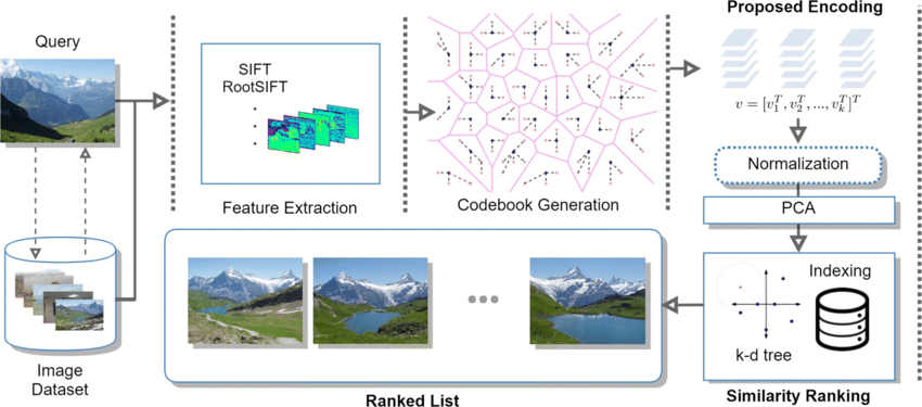
Semantic Similarity Search and Vector Databases
Embeddings are a key part of modern searches that seek meaning, rather than matching exact words.
A user's query (whether it's a text description or another image) and the items in your database (documents or images) are turned into the same vector space.
The search engine then finds the items whose vectors are closest to the query's vector. Storing these vectors in a vector database makes searching quick and efficient, even with millions of items.
Retrieval-Augmented Generation (RAG) in LLMs
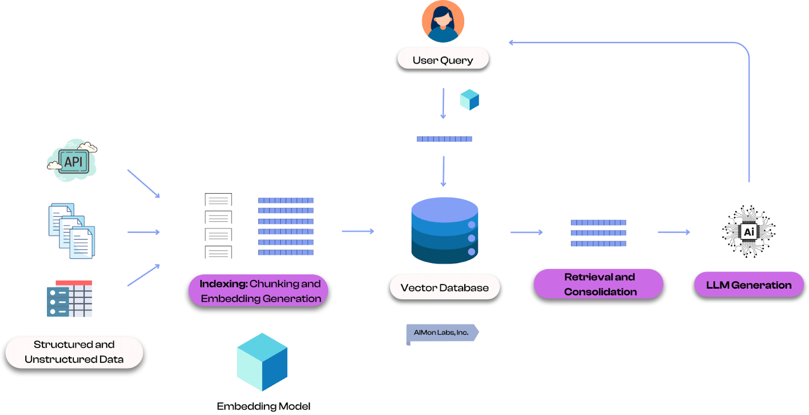
Large language models (LLMs) are powerful, but their knowledge is often limited to the data they were trained on. RAG allows language models to use embeddings to retrieve relevant information for user queries.
When a user asks a question, the question is first embedded into a vector. Then it is used to find relevant information from a database, which is then fed to the LLM to generate a more accurate and up-to-date answer.
Recommendation Systems
Recommendation systems create vector representations for both users and items in a shared embedding space.
These systems can accurately predict and recommend content or products users are likely to enjoy or buy by finding items with high semantic similarity to their query vector.

Active Learning and Data Selection
Real-life datasets often contain duplicates or overly similar samples that waste labeling budgets and reduce diversity. Active learning is a strategy for intelligently selecting the most valuable data to label, and embeddings are key to making it work.
One common strategy is diversity sampling, which uses embeddings to cluster unlabeled data. Then select a few samples from each cluster to ensure the data for labeling is varied and representative.
LightlyOne helps with this by offering the DIVERSITY strategy.
 "strategies": [
            {
                "input": {
                    "type": "EMBEDDINGS"
                },
                "strategy": {
                    "type": "DIVERSITY"
                }
            }
        ]
DIVERSITY strategy also includes a setting called stopping_condition_minimum_distance that prevents the selection of samples that are too similar and maximizes the impact of your labeling budget.
"strategy": {
    "type": "DIVERSITY",
    "stopping_condition_minimum_distance": 0.2,
    "strength": 0.6 # optional
}
Best Practices and Considerations for Using Embeddings
When using embeddings in machine learning, keep these considerations in mind, so you can get the most out of embeddings:
- Choose the Right Embedding Model: Match the model to your task and resources. Static embeddings (Word2Vec) are lightweight, while contextual models (BERT) offer richer meaning but require more compute. Also, match the models to your data, like CNN for images, transformer for text,and graph neural models for networks.
- Dimensionality and Efficiency: The specified dimension of your embedding vector is a trade-off. Higher dimensions capture more detail but are slower and risk overfitting. Lower dimensions are faster but may be less precise. Start with a common dimension and then adjust it based on validation and the resource budget.
- Normalization: For accurate and fast similarity calculations, always normalize your vectors to a unit length. It allows you to use the dot product, which is computationally cheaper than cosine similarity.
- Bias and Ethics: Embeddings learn and can amplify biases from your training data. Address this by using debiasing techniques or carefully curating training data with active learning. Utilize LightlyOne to scale active learning and curate training data that helps reduce bias.
- Debugging and Evaluation: Always verify embeddings by checking sample vectors' nearest neighbors for relevance. If embeddings are not grouping things logically, the training might need adjustment. Intrinsic tests (word analogies, categorization) and downstream validation (model performance) help evaluate quality.
Here’s a quick-reference table summarizing the different types of embeddings, their models, and use cases.
How Can Lightly AI Help With Your Embedding Requirements?
Obtaining high-quality embeddings depends on both the model you choose and the data you use to train it. While public datasets provide a good starting point, they often overlook the unique patterns in your domain and limit the model's performance.
LightlyOne solves the data problem by ensuring you train on the best possible data. It analyzes your unlabeled data to pick a diverse and meaningful subset that covers key scenarios.
This high-impact dataset is then used to pre-train an embedding model with LightlyTrain. It creates a custom model using self-supervised learning methods like SimCLR and DINOv2.
Pre-training teaches your model the specific visual features and patterns of your domain before you even begin fine-tuning with labels. And it leads to higher performance on downstream tasks.
Conclusion
Embeddings are a way to turn complicated data into numbers (numerical language) that ML models can understand. They take things from the real world and convert them into numbers, and similar items end up close to each other in embedding space. Whether you’re working with pre-trained models or training your own, embeddings bridge the gap between real-world data and machine understanding.

Stay ahead in computer vision
Get exclusive insights, tips, and updates from the Lightly.ai team.


.png)
.png)
.png)


