Predicting Rain from Satellite Images (Part 1)
Table of contents
Can a neural network predict rain from satellite images? Part 1: Data collection and analysis
Can satellite images predict rainfall? Here’s how we started.

What’s the challenge?
Predicting precipitation in data-sparse regions using only satellite imagery.
Who’s involved?
Meteomatics, a weather API provider, teamed up with us to test a neural network approach.
What data did we collect?
Quarter-hourly infrared satellite images (Europe, North America, Mexico) plus ground-truth rainfall data (Europe & North America).
What did we discover during analysis?
- Regional images form distinct clusters (good for testing generalization).
- Many redundant images due to short collection period.
How did we curate the dataset?
Using LightlyOne’s coreset sampling, reducing the European training set from 1158 to 578 diverse images.
Introduction
Predicting and understanding weather has become crucial in a number of industries, including agriculture, autonomous driving, aviation, or the energy sector. For example, weather conditions play a significant role for aviation and logistics companies in planning the fastest and safest route. Similarly, renewable energy companies need to be able to predict the amount of energy they will produce at a given day. As a consequence various weather models have been developed and are being applied all over the world. Unfortunately, these models often require highly specific information about the atmosphere and exact conditions.
For this reason, Meteomatics, a weather API that delivers fast, direct and simple access to an extensive range of global weather, climate projections and environmental data, has reached out to us for help. Their goal: To predict precipitation accurately in regions where data is sparse and they have to rely on satellite imagery. In this blog post, we show how we developed a neural network to predict the amount of rainfall in a given region based on infrared satellite data.
This is part one of a two-part blog:
- Part 1: Data Collection and Analysis
- Part 2: Method and Results
Data collection and analysis
If you have ever worked with neural networks you know that they can be data hungry. For this reason it’s crucial to set up a data pipeline that allows you to collect, manage, and understand the assembled data. Our collaboration partner, Meteomatics, offers an easy-to-use API which enables us to quickly gather training and ground-truth data. For example, to get an infra-red picture of Europe (coordinates from 65, -15 to 35, 20) on the seventh of July 2021 and at a resolution of 800x600 pixels we can simply make the following query:
We ran a Python script every quarter hour for a few days collecting infra-red images over Europe, North America, and Mexico at different wavelengths. We then locally combined the different images for each timestamp into an RGB image. To make the task easier we masked out stratiform precipitation in a first step. However, as we will see later on, this only has a small effect on the accuracy of the model. We also collected ground-truth data for training and evaluating the accuracy of our model. Note that ground-truth data was only available for Europe and North America. Below you can see a pair of input and ground-truth data over Europe:
💡 Pro Tip: For satellite imagery pipelines that rely on heavy preprocessing, We switched from Pillow to Albumentations and got 2x speedup explains how optimizing augmentation libraries can significantly reduce end to end experiment time.

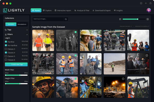
Following the notorious “garbage in garbage out” mantra, we wanted to understand and curate the collected data before we trained a machine learning algorithm on it. For this, we used our free-to-use exploration tool LightlyOne. LightlyOne enables quick and easy ways to analyze a dataset as well as more in-depth algorithms to pick the most relevant training points. After uploading our dataset to LightlyOne we immediately noticed a crucial property of the collected data: The images over Europe, North America, and Mexico were visually and semantically separated. This resulted in a simple strategy to test the generalization capacity of the algorithm: If we trained it on the data from Europe and it performed well on unseen data from North America and Mexico, the algorithm would generalize well. Note that if we had picked the training dataset and the test dataset to be very similar, then all we would test is the memory of the neural network.

Another key insight we gained was that there were many small clusters of extremely similar images. This is due to the fact that we collected data over a relatively short period of time. Because of this, there were a lot of similar images in the dataset which made it harder for the model to generalize well. LightlyOne helped us with removing these redundancies with a method called “coreset sampling” which aims to maximize the diversity of the dataset.
💡Pro tip: For domains with scarce labels, our Self-Supervised Learning for Medical Imaging article illustrates how SSL learns strong representations without manual annotation.
Before curating the dataset with LightlyOne, we had 1158 images in our training dataset (Europe). After data curation, we are left with 578 images. The validation dataset (North America) consists of 1107 images and the test dataset (Mexico) consists of only 43 images as we began data collection later.
We download the images from LightlyOne and and now we are ready to do some machine learning. Head to Part 2 to see the results!
See Lightly in Action
Curate and label data, fine-tune foundation models — all in one platform.
Book a Demo

Stay ahead in computer vision
Get exclusive insights, tips, and updates from the Lightly.ai team.


.png)
.png)
.png)


