Which Optimizer should I use for my ML Project?

This article provides a summary of popular optimizers used in computer vision, natural language processing, and machine learning in general. Additionally, you will find a guideline based on three questions to help you pick the right optimizer for your next machine learning project.

TL;DR:
1) Find a related research paper and start with using the same optimizer.
2) Consult Table 1 and compare properties of your dataset to the strengths and weaknesses of the different optimizers.
3) Adapt your choice to the available resources.

‍

Introduction

Choosing a good optimizer for your machine learning project can be overwhelming. Popular deep learning libraries such as PyTorch or TensorFLow offer a broad selection of different optimizers — each with its own strengths and weaknesses. However, picking the wrong optimizer can have a substantial negative impact on the performance of your machine learning model [1][2]. This makes optimizers a critical design choice in the process of building, testing, and deploying your machine learning model.

The problem with choosing an optimizer is that, due to the no-free-lunch theorem, there is no single optimizer to rule them all; as a matter of fact, the performance of an optimizer is highly dependent on the setting. So, the central question that arises is:

Which optimizer suits the characteristics of my project the best?

The following article is meant as a guide to answering the question above. It is structured into two main paragraphs: In the first part, I will present to you a quick introduction to the most frequently used optimizers. In the second part, I will provide you with a three-step plan to pick the best optimizer for your project.

‍

Frequently Used Optimizers

Almost all popular optimizers in deep learning are based on gradient descent. This means that they repeatedly estimate the slope of a given loss function L and move the parameters in the opposite direction (hence climbing down towards a supposed global minimum). The most simple example for such an optimizer is probably stochastic gradient descent (or SGD) which has been used since the 1950s [3]. In the 2010s the use of adaptive gradient methods such as AdaGrad or Adam [4][1] has become increasingly popular. However, recent trends show that parts of the research community move back towards using SGD over adaptive gradient methods, see for example [2] and [5]. Furthermore, current challenges in deep learning bring rise to new variants of SGD like LARS or LAMB [6][7]. For example, Google Research use LARS to train a powerful self-supervised model in one of their latest papers [8].

The section below will be an introduction to the most popular optimizers. Head to section How to Choose the Right Optimizer if you are already familiar with the concepts.

We will use the following notation: Denote by w the parameters and by g the gradients of the model. Furthermore, let α be the global learning rate of each optimizer and t the time step.

Stochastic Gradient Descent (SGD) [9]

In SGD, the optimizer estimates the direction of steepest descent based on a mini-batch and takes a step in this direction. Because the step size is fixed, SGD can quickly get stuck on plateaus or in local minima.

SGD with Momentum [10]

Where β < 1. With momentum, SGD accelerates in directions of constant descent (that’s why it’s also called the “heavy ball method”). This acceleration helps the model escape plateaus and makes it less susceptible to getting stuck in local minima.

AdaGrad (2011, [4])

AdaGrad is one of the first successful methods which makes use of adaptive learning rates (hence the name). AdaGrad scales the learning rate for each parameter based on the square root of the inverse of the sum of the squared gradients. This procedure scales sparse gradient directions up which in turn allows for larger steps in these directions. The consequence: AdaGrad can converge faster in scenarios with sparse features.

RMSprop (2012, [11])

RMSprop is a non-published optimizer which has been used excessively in the last years. The idea is similar to AdaGrad but the rescaling of the gradient is less aggressive: The sum of squared gradients is replaced by a moving average of the squared gradients. RMSprop is often used with momentum and can be understood as an adaption of Rprop to the mini-batch setting.

Adam (2014, [1])

Adam combines AdaGrad, RMSprop and momentum methods into one. The direction of the step is determined by a moving average of the gradients and the step size is approximately upper bounded by the global step size . Furthermore, each dimension of the gradient is rescaled similar to RMSprop. One key difference between Adam and RMSprop (or AdaGrad) is the fact that the moment estimates m and v are corrected for their bias towards zero. Adam is well-known for achieving good performance with little hyper-parameter tuning.

AdamW (2017, [17])

Loshchilov and Hutter [17] identified the inequivalence of L2 regularization and weight-drop in adaptive gradient methods and hypothesized that this inequivalence limits Adams performance. They then proposed to decouple the weight decay from the learning rate. The empirical results show that AdamW can have better generalization performance than Adam (closing the gap to SGD with momentum) and that the basin of optimal hyperparameters is broader for AdamW.

LARS (2017, [6])

LARS is an extension of SGD with momentum which adapts a learning rate per layer. It has recently caught attention in the research community. The reason is that due to the steadily growing amount of available data, distributed training of machine learning models has gained popularity. The consequence is that batch sizes begin growing. However, this leads to instabilities during training. Yang et al. [6] argue that these instabilities stem from an imbalance between the gradient norm and the weight norm for certain layers. They therefore came up with an optimizer which rescales the learning rate for each layer based on a “trust” parameter η < 1 and the inverse norm of the gradient for that layer.

‍

How to Choose the Right Optimizer

As mentioned above, choosing the right optimizer for your machine learning problem can be hard. More specifically, there is no one-fits-all solution and the optimizer has to be carefully chosen based on the particular problem at hand. In the following section I will propose three questions you should ask yourself before deciding to use a certain optimizer.

What are the state-of-the-art results on datasets and tasks similar to yours? Which optimizers were used and why?

If you are working with novel machine learning methods, odds are there exist one or more reliable papers which cover a similar problem or handle similar data. Oftentimes the authors of the paper have done extensive cross-validation and report only the most successful configurations. Try to understand the reasoning for their choice of optimizer.

Example: Say you want to train a Generative Adversarial Network (GAN) to perform super-resolution on a set of images. After some research you stumble upon this [12] paper in which the researchers used the Adam optimizer to solve the exact same problem. Wilson et al. [2] argue that training GANs does not correspond to solving optimization problems and that Adam may be well-suited for such scenarios. Hence, in this case, Adam is a good choice for an optimizer.

Are there characteristics to your dataset which play to the strengths of certain optimizers? If so, which ones and how?

Table 1 shows an overview of the different optimizers with their strengths and weaknesses. Try to find an optimizer which matches the characteristics of your dataset, training setup, and goal of the project.

Certain optimizers perform extraordinarily well on data with sparse features [13] and others may perform better when the model is applied to previously unseen data [14]. Some optimizers work very well with large batch sizes [6] while others will converge to sharp minima with poor generalization [15].

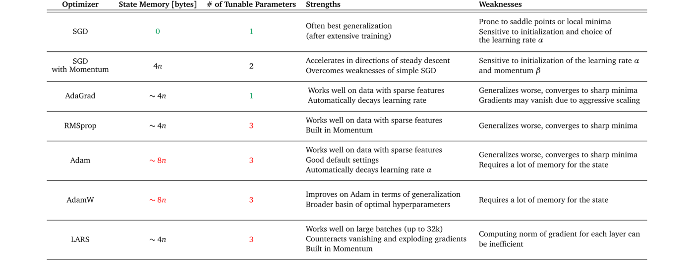
Example: For a project at your current job you have to classify written user responses into positive and negative feedback. You consider to use bag-of-words as input features for your machine learning model. Since these features can be very sparse you decide to go for an adaptive gradient method. But which one do you want to use? Consulting Table 1, you see that AdaGrad has the fewest tunable parameters of the adaptive gradient methods. Seeing the limited time frame of your project you choose AdaGrad as an optimizer.

What are your resources for the project?

The resources which are available for a project also have an effect on which optimizer to pick. Computational limits or memory constraints, as well as the time frame of the project can narrow down the set of feasible choices. Looking again at Table 1, you can see the different memory requirements and number of tunable parameters for each optimizer. This information can help you estimate whether or not the required resources of an optimizer can be supported by your setup.

Example: You are working on a project in your free-time in which you want to train a self-supervised model (e.g. SimCLR [16]) on an image dataset on your home computer. For models like SimCLR, the performance increases with an increased batch size. Therefore, you want to save as much memory as possible so that you can do training in large batches. You choose a simple stochastic gradient descent without momentum as your optimizer because, in comparison to the other optimizers, it requires the least amount of additional memory to store the state.

‍

Conclusion

Trying out all possible optimizers to find the best one for a project is not always possible. In this blog post I provided an overview over the update rules, strengths, weaknesses, and requirements of the most popular optimizers. Furthermore, I listed three questions to guide you towards making an informed decision about which optimizer to use for your machine learning project.

As a rule of thumb: If you have the resources to find a good learning rate schedule, SGD with momentum is a solid choice. If you are in need of quick results without extensive hypertuning, tend towards adaptive gradient methods.

I hope that this blog post will serve as a helpful orientation and that I could assist one or the other in making the right optimizer choice.

I am open for feedback, let me know if you have any suggestions in the comments!

Philipp Wirth
Machine Learning Engineer at Lightly

‍

Changelog:

• 17.12.2020: Added AdamW.

‍

[1]: Kingma, D. P. & Ba, J. (2014), ‘Adam: A Method for Stochastic Optimization’ , cite arxiv:1412.6980Comment: Published as a conference paper at the 3rd International Conference for Learning Representations, San Diego, 2015 .

[2]: Wilson, Ashia C. et al. “The Marginal Value of Adaptive Gradient Methods in Machine Learning.” ArXiv abs/1705.08292 (2017): n. pag.

[3]: Robbins, Herbert; Monro, Sutton. A Stochastic Approximation Method. Ann. Math. Statist. 22 (1951), no. 3, 400–407. doi:10.1214/aoms/1177729586. https://projecteuclid.org/euclid.aoms/1177729586

[4]: Duchi, J. C.; Hazan, E. & Singer, Y. (2011), ‘Adaptive Subgradient Methods for Online Learning and Stochastic Optimization.’, J. Mach. Learn. Res. 12 , 2121–2159.

[5]: Keskar, Nitish Shirish and Richard Socher. “Improving Generalization Performance by Switching from Adam to SGD.” ArXiv abs/1712.07628 (2017): n. pag.

[6]: You, Yang et al. (2017) ‘Large Batch Training of Convolutional Networks.’ arXiv: Computer Vision and Pattern Recognition (2017): n. pag.

[7]: You, Yang et al. “Large Batch Optimization for Deep Learning: Training BERT in 76 minutes.” arXiv: Learning (2020): n. pag.

[8]: Grill, Jean-Bastien et al. “Bootstrap Your Own Latent: A New Approach to Self-Supervised Learning.” ArXiv abs/2006.07733 (2020): n. pag.

[9]: Bharath, B., Borkar, V.S. Stochastic approximation algorithms: Overview and recent trends. Sadhana 24, 425–452 (1999). https://doi.org/10.1007/BF02823149

[10]: David E. Rumelhart, Geoffrey E. Hinton, and Ronald J. Williams. 1988. Learning representations by back-propagating errors. Neurocomputing: foundations of research. MIT Press, Cambridge, MA, USA, 696–699.

[11]: Tieleman, T. and Hinton, G., 2012. Lecture 6.5-rmsprop: Divide the gradient by a running average of its recent magnitude. COURSERA: Neural networks for machine learning, 4(2), pp.26–31.

[12]: C. Ledig et al., “Photo-Realistic Single Image Super-Resolution Using a Generative Adversarial Network,” 2017 IEEE Conference on Computer Vision and Pattern Recognition (CVPR), Honolulu, HI, 2017, pp. 105–114, doi: 10.1109/CVPR.2017.19.

[13]: John Duchi, Elad Hazan, and Yoram Singer. 2011. Adaptive Subgradient Methods for Online Learning and Stochastic Optimization. J. Mach. Learn. Res. 12, null (2/1/2011), 2121–2159.

[14]: Moritz Hardt, Benjamin Recht, and Yoram Singer. 2016. Train faster, generalize better: stability of stochastic gradient descent. In Proceedings of the 33rd International Conference on International Conference on Machine Learning — Volume 48(ICML’16). JMLR.org, 1225–1234.

[15]: Keskar, Nitish Shirish et al. “On Large-Batch Training for Deep Learning: Generalization Gap and Sharp Minima.” ArXiv abs/1609.04836 (2017): n. pag.

[16]: Chen, Ting et al. “A Simple Framework for Contrastive Learning of Visual Representations.” ArXiv abs/2002.05709 (2020): n. pag.

[17]: Loshchilov and Hutter “Decoupled Weight Decay Regularization” ArXiv abs/1711.05101 (2017)

‍